


Tutorial 14: System Identification of a Franka#
Note
The System Identification extension is in beta. Its workflow, run contracts, exported run specifications, and APIs are not guaranteed to stay future compatible.
This tutorial runs a reproducible, free-space system-identification experiment for a fixed-base Franka Panda. To make the optimization behavior visible, it begins with a deliberately over-frictional working asset. The source asset is preserved; only a separate tutorial overlay is degraded. After recovering joint friction, the tutorial diagnoses the remaining held-out residual and runs a separately bounded joint-damping phase. Each phase starts from the previously persisted candidate and must pass its own replay gate.
The example uses recorded MCAP telemetry, explicit command alignment, separate training and validation motions, Newton MuJoCo rollouts, and CMA-ES. Optimization, USD mutation, replay, and promotion remain separate operations so that every stage is reviewable and reversible.

The walkthrough follows the same progression: reference excitation and telemetry on the left, the deliberately poor initial model in orange, and the recovered candidate in green.#
After completing this tutorial, you will be able to:
Construct a controlled poor initialization without modifying a source asset.
Validate telemetry mapping, timing, excitation, and effort semantics.
Configure and export a bounded friction-only RunSpec.
Solve, persist, and independently replay one parameter phase.
Diagnose held-out residuals and configure a conservative second phase.
Compare candidates with a predeclared acceptance policy.
Decide when to promote a candidate and when to collect new excitation data.
Interpret predictive improvement without overstating physical identifiability.
For the complete feature reference, see System Identification Extension.
60-80 minute tutorial, excluding optimization time
Reference outcome#
The tutorial intentionally authors an excessive 1.0 N*m*s/rad of Newton joint friction on all seven arm joints in a working overlay before fitting. The independently reloaded friction candidate reduces held-out normalized cost by 42.7%. Position, velocity, and torque RMSE improve by 8.3%, 13.7%, and 24.4%, respectively.
A second phase opens only seven joint-damping scales. Its independently reloaded candidate reduces torque RMSE from 1.6573 N*m to 1.3946 N*m and normalized cost by another 28.9%. Position and velocity RMSE regress slightly relative to the friction candidate, by 2.0% and 1.1%, while remaining better than the poor seed. The final decision therefore demonstrates an explicit application tradeoff instead of selecting the lowest scalar objective without review.
This is a stress-test initialization, not a recommended engineering prior. It demonstrates a staged tuning cycle from a meaningfully poor model while keeping every experiment stable and reviewable.
Prerequisites#
A built NVIDIA Isaac Sim source checkout.
isaacsim.robot_setup.sysid.uienabled. Open Window > Extensions, search for system identification, and enableisaacsim.robot_setup.sysid.ui. The interactive extension automatically enables theisaacsim.robot_setup.sysidbackend.The packaged Franka tutorial from the Content Browser at
IsaacSim/Samples/SystemIdentification/franka_sysid_tutorial/. Use these exact paths:Stage:
assets/franka_poor_seed.usda, which references the packaged source assetassets/franka.usda. Copy both.RunSpec:
config/franka_friction_run_spec.json.MCAP recording:
data/bag_0.mcap.Topic mapping:
data/franka_sysid_topic_map.yaml.Collection manifest:
data/collection_manifest.json.Reference result:
results/franka_friction_result.json.
The fixed-base stage articulation resolves to
/World/envs/env_0/panda_instanceable.A CUDA-capable GPU for the Newton MuJoCo population rollout.
A local working directory for RunSpecs, reports, checkpoints, and output USDs. Copy the complete
franka_sysid_tutorialdirectory and preserve its packaged subdirectory layout, because the packaged RunSpec resolves../assets,../data, and../resultsrelative to its own location underconfig/. Then add one emptyrunssubdirectory for everything this tutorial generates. Do not modify the Samples originals.This tutorial refers to that working directory as
C:\sysid_tutorialon Windows and~/sysid_tutorialon Linux:sysid_tutorial/ |-- assets/ franka_poor_seed.usda, franka.usda (packaged inputs) |-- config/ franka_friction_run_spec.json (packaged reference) |-- data/ bag_0.mcap, topic map, manifest (packaged inputs) |-- results/ franka_friction_result.json (packaged reference) `-- runs/ everything you export, solve, apply, and replay
The reference recording contains 9,439 samples for seven arm joints at approximately 30 Hz. It provides joint position, velocity, command, and link-side torque.
Important
System Identification consumes excitation data; it does not generate or certify safe robot commands. Validate joint, velocity, acceleration, effort, collision, and workspace limits before executing a trajectory on hardware. See Trajectory generation and excitation for external experiment-design resources.
Step 1: Open the deliberately poor working asset#
Copy the complete IsaacSim/Samples/SystemIdentification/franka_sysid_tutorial/ directory into your
working directory as described in Prerequisites, then open assets/franka_poor_seed.usda and confirm
that the articulation initializes. The packaged stage already carries the over-frictional values below, so
there is nothing to author here; the table records what was degraded and why. Do not edit the Samples
originals.
franka_poor_seed.usda is a thin overlay over the packaged assets/franka.usda, which it references
rather than edits. The source asset authors no Newton joint friction at all, so every arm joint would
otherwise run at the solver default. The overlay selects the Newton physics variant and raises all seven
arm joints to 1.0 N*m*s/rad, leaving stiffness, damping, armature, masses, inertias, and controller
settings untouched. That isolates the injected error to the single family the tutorial optimizes.
Property |
Source asset |
Poor working overlay |
|---|---|---|
Joint 1-7 Newton friction |
Not authored |
1.0 N*m*s/rad |
Other physical properties |
Unchanged |
Unchanged |
Friction is authored as newton:friction under NewtonJointAPI. That is the attribute both the Newton
solver and System Identification read; a plain jointFriction value is inert to both.
The poor seed remains numerically stable, but its excess friction creates a measurable trajectory and torque mismatch. This controlled construction is preferable to changing several coupled families at once because the cause of the initial error is known.
Warning
The 1.0 N*m*s/rad seed is a deliberately excessive tutorial value, not a measurement of a physical Franka, and the recording carries no authored friction value for the optimizer to rediscover. The recovered result is evaluated as a better predictive model for this recording, not as a certificate of true joint friction.
Step 2: Select the robot and configure the rollout#
With isaacsim.robot_setup.sysid.ui enabled, open Tools > Robotics > Asset Editors >
System Identification. The panel is a six-stage workflow: 1 Robot, 2 Data, 3 Parameters,
4 Check, 5 Solve, and 6 Results. Work through the stages in that order. Select a stage from the
tab strip at the top of the panel, or use Back and Next at the bottom.
On 1 Robot, at the top of the tab:
Set Physics engine to
Newton (MuJoCo).Set Robot prim path to
/World/envs/env_0/panda_instanceable. The field defaults to/World/envs/env_0, which is the environment prim rather than the articulation, so type the full path.
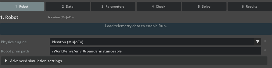
The list pairs an engine with a solver rather than offering the two separately. Both Newton entries
are the same engine with a different solver, so picking Newton (MuJoCo) chooses Newton and its
MuJoCo solver in one step.#
Important
Physics engine does not change the physics runtime of the running application. Selecting
Newton (MuJoCo) does not migrate your stage to Newton, does not rewrite the stage’s
PhysicsScene, and does not alter how the robot behaves when you press Play. The viewport and
the timeline keep using whatever physics the stage is already configured for.
What the setting does control is which engine the System Identification job simulates its candidate
parameters on, both for the panel’s own Run on 5 Solve and through the simulation.engine
key of the RunSpec you export in Step 7, which the headless tools in Steps 8 through 15 consume.
It also feeds several things inside the panel, so treat it as a decision to make before you configure
the rest of the run rather than one to revisit later. It is part of the check signature, so changing
it invalidates a completed 4 Check the same way the Step 7 solver settings do. It decides whether
the Newton block below is shown at all, drives the backend-compatibility hint on 5 Solve, and
determines whether the timeline has to be playing: only Isaac Sim (in-app) requires it, so the
Newton rollouts in this tutorial run without pressing Play.
Expand Advanced simulation settings and set the Newton rollout controls:
Setting |
Reference value |
|---|---|
Newton device |
|
Controller |
|
Controller feedforward |
|
Effort clamp |
|
CUDA graph capture |
Selected (default) |
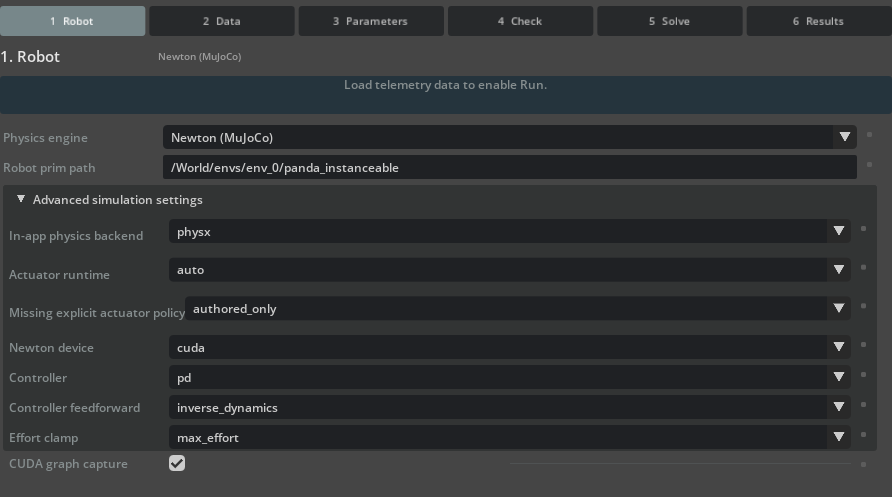
The Newton block appears only while Physics engine is a Newton selection.#
Leave In-app physics backend and Missing explicit actuator policy at their defaults; they apply to
the Isaac Sim (in-app) engine. Leave Actuator runtime at auto, which resolves to mixed actuator
ownership for standalone MuJoCo. The Offline stepping control and the clone settings are hidden for this
run because they belong to the Isaac Sim (in-app) engine; the equivalent RunSpec key is
simulation.offline_stepping.
Newton MuJoCo supports batched, derivative-free population evaluation. The differentiable Newton Featherstone rollout is a separate headless-only path with a narrower supported parameter set; it is not used by this CMA-ES walkthrough.
Leave CUDA graph capture enabled for repeated, fixed-shape CMA-ES evaluations. The first evaluation warms the kernels and solver storage, the next captures that shape, and later evaluations reuse the graph. Each captured and uncaptured MuJoCo rollout resets rollout-local warm-start, actuator-activation, applied-force, and control buffers before restoring the initial joint state, so a preceding candidate batch does not seed the next one.
In a reference Franka run with 16 candidates and 800 steps, graph replay reduced median evaluation time from 13.59 seconds uncaptured to 0.515 seconds captured, a 26.4x speedup after warmup. The ratio is specific to that workload and hardware. For a new stage or RunSpec, compare a captured result with an uncaptured result using declared numerical tolerances. Small GPU floating-point differences are expected; disable capture if the difference exceeds the acceptance threshold rather than requiring bitwise equality.
Step 3: Load and verify telemetry#
Select 2 Data. The source fields sit at the top of the tab, above Load Trajectory.
The Command alignment (s) field belongs to this group because changing it forces a reload. The telemetry diagnostic estimates a common timing offset between commands and measured response, and the reference recording produced:
Diagnostic |
Value |
|---|---|
Common lag (samples) |
16.0825 |
Common lag (seconds) |
0.536075 |
Joint-to-joint residual spread |
0.5336 samples |
Those numbers come from an uncorrected load. To measure them yourself rather than taking them on faith, leave Command alignment (s) at its default of 0 for a first Load Trajectory, read the diagnostic, and then enter the offset and reload. The steps below go straight to the corrected load.
Set Source type to
MCAP.Set Data source path to your local copy of
data/bag_0.mcap.Set Mapping config to
data/franka_sysid_topic_map.yaml.Set Chunk manifest to
data/collection_manifest.json.Set Command alignment (s) to
0.5360748729665944.Click Load Trajectory.
Enter all sixteen digits. The field displays four decimals, so it will read 0.5361 after you commit it,
but it stores and exports the full value.
Command alignment corrects the recorded series before fitting. Actuator command delay changes the simulated model, so leave the actuator command-delay parameter disabled for this phase. Applying both to the same logging offset would double-count the effect.
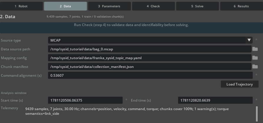
Analysis window autofills to the full recording span, and the Telemetry summary reports the sample count, channels, and torque semantics.#
Confirm that the Telemetry summary reads 9439 samples, 7 joints, 30.00 Hz, lists
channels=position, velocity, command, torque, and ends with torque semantics=link_side. The
torque-semantics field matters because motor-side, link-side, commanded, and measured efforts are not
interchangeable. Also verify joint order, signs, units, timestamp gaps, clipping, and long flat intervals.
The summary also reports 1 warning(s) at this point, and the stage header reads 1 train / 0
validation chunk(s). Both describe the same condition: no validation holdout is configured yet. Step 4
resolves it.
Step 4: Separate training and validation#
Stay on 2 Data and scroll to Dataset partitioning.
Under Automatic validation holdout, leave Enabled cleared. It is cleared by default, and manual chunks take precedence over the automatic holdout in any case.
The packaged recording ships a collection manifest but no phase_events.jsonl companion, so no phase
chunks are imported and Configured manual chunks starts empty. Enter the two tutorial motions with the
Manual chunk editor. Add Chunk captures whatever is currently in Analysis window, so set the
window first for each chunk:
Name |
Role |
Excitation |
Start time (s) |
End time (s) |
|---|---|---|---|---|
|
Train |
|
1781120740.1658437 |
1781120763.886561 |
|
Validation |
|
1781120792.565396 |
1781120819.9389462 |
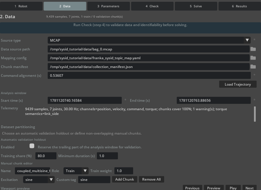
Analysis window holds the training chunk bounds while the Manual chunk editor carries its name, role, and excitation tag.#
For each row, set Start time (s) and End time (s) in Analysis window, then set Name,
Role, and Excitation in Manual chunk editor, then click Add Chunk. After adding both
chunks, set Analysis window to span them both: 1781120740.1658437 to 1781120819.9389462. The
exported RunSpec stores that span as telemetry.time_window, and the reference results later in this
tutorial were produced with it.

The chunk table snaps each requested window to sample boundaries: 711 samples over 23.667 s for the training chunk and 821 samples over 27.333 s for the validation chunk.#
The training multisine contributes to the optimizer. The validation multisine is withheld from optimization and is used for model selection and the final replay. Both motions exercise all seven joints, but they do not guarantee that every selected physical parameter is independently identifiable.
Step 5: Select the friction parameter phase#
Select 3 Parameters.
Expand Additional parameter families and select Edit bounds (Initial/Min/Max). The parameter table replaces its single Value column with Initial, Min, and Max columns.
Under Parameters to identify, click Friction in the Families row. This selects the friction row of every joint and targets that family for bulk bounds.
In Family bounds, enter
1.0for Initial,0.1for Min, and1.5for Max, then click Apply.
Family |
Count |
Initial |
Minimum |
Maximum |
|---|---|---|---|---|
Joint friction |
7 |
1.0 |
0.1 |
1.5 |
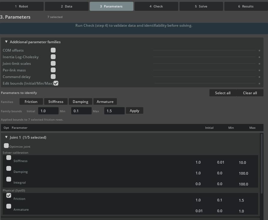
Each joint group separates Solver calibration rows (stiffness, damping, integral) from Physical (SysID) rows (friction, armature).#
Confirm that the stage header reads 7 selected and that the status line under Family bounds reads
Applied bounds to 7 selected friction rows. Expand a joint group to verify that its Friction row
carries 1.0, 0.1, and 1.5.
The scale value 1.0 represents the deliberately poor 1.0 N*m*s/rad property carried by the poor-seed overlay from Step 1. The bounds therefore correspond to 0.1-1.5 N*m*s/rad on this working asset.
Do not add stiffness, damping, or armature to this first phase simply because the UI permits it. Adding coupled families would make a larger numerical improvement harder to interpret and would no longer match the controlled error introduced in Step 1. The later damping phase starts only after the friction candidate has been persisted, replayed, and accepted as its own baseline.
Step 6: Run the identifiability check#
Select 4 Check and click Run Check.
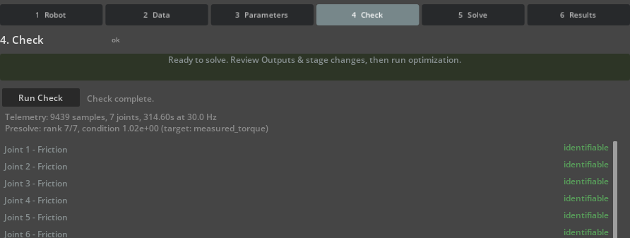
For the friction phase, a green banner and an ok stage badge mean the run gate is satisfied. Scroll
the verdict list to see all seven joints.#
At this point the friction-only regressor reports rank 7/7, condition 1.04e+00 (target:
measured_torque), and all seven rows return identifiable. A count such as 7 selected is not an
identifiability result; use the per-parameter verdicts, rank, conditioning, and sensitivity instead.
Note
Re-running the check after Step 7 reports condition 1.02e+00 instead. The cause is Max rollout
steps, which Step 7 raises from its default of 300 to 800: the presolve regresses over that many
samples per chunk, so the check here fits 300 of the 711 training samples while the Step 7 re-run fits
all of them. Both results are correct for their own sample count, and neither changes the verdicts.
Step 7: Configure the optimizer and export#
Select 5 Solve. Set the three controls at the top of the tab, then expand Advanced solver settings for the rest:
Section |
Setting |
Reference value |
|---|---|---|
Top of tab |
Optimizer |
CMA-ES |
Top of tab |
Max iterations |
48 |
Top of tab |
Max rollout steps |
800 |
Advanced solver settings |
CMA-ES sigma |
0.2 |
Advanced solver settings |
CMA-ES batch size |
16 |
Advanced solver settings |
CMA-ES seed |
20260730 |
Advanced solver settings |
Weight: position |
1.0 |
Advanced solver settings |
Weight: velocity |
1.0 |
Advanced solver settings |
Weight: torque |
0.01 |
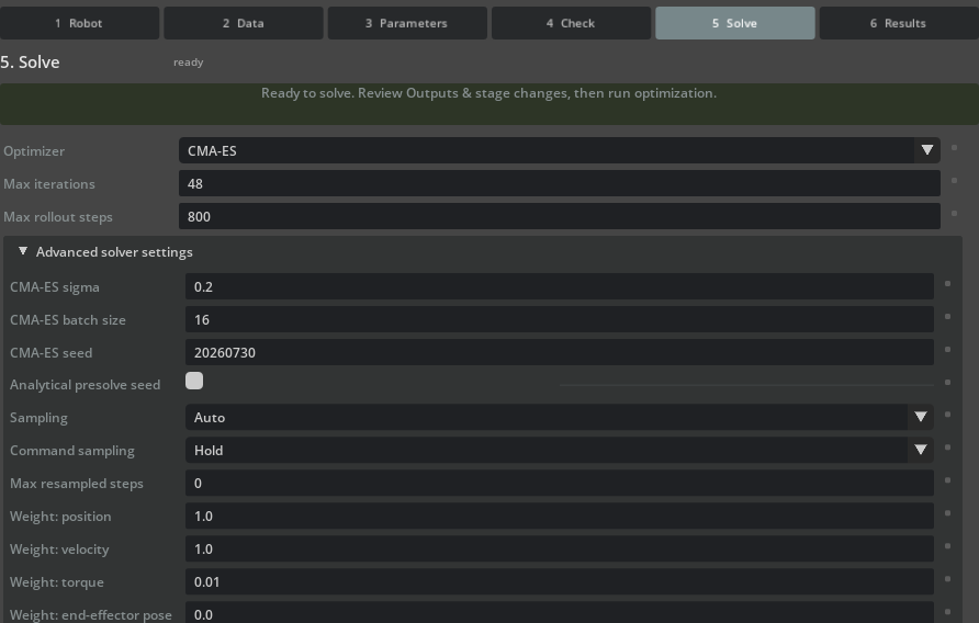
CMA-ES batch size caps how many candidates are evaluated per rollout wave. There is no population field: CMA-ES derives its population from the number of optimized parameters.#
Now return to 4 Check and click Run Check once more. Three of the settings above belong to the
check signature and invalidated the Step 6 result when you changed them: Optimizer, Max rollout
steps, and the three residual weights. Max iterations, CMA-ES sigma, CMA-ES batch size, and
CMA-ES seed are not part of the signature and leave an existing check valid. For the friction phase the
5 Solve stage badge changes from not ready to ready once the check passes again.
Back on 5 Solve, scroll to Outputs & stage changes and click Export RunSpec. Save it as
franka_friction_run_spec.json in the runs subdirectory of your working directory. The packaged
config/franka_friction_run_spec.json is a reference copy for comparison; every command in this
tutorial reads the one you just exported from runs.
Note
One key the reference uses has no control in the panel: solver.cma_population_size. The packaged
RunSpec sets it to 16, while a GUI export leaves it unset. CMA-ES then derives its population from the
seven optimized parameters, which yields 9, and CMA-ES batch size clamps to that same 9. To
reproduce the iteration count and recovered scales reported below, open the exported file and add
"cma_population_size": 16 to its solver section. This is the same RunSpec-only situation as
simulation.offline_stepping in Step 2.
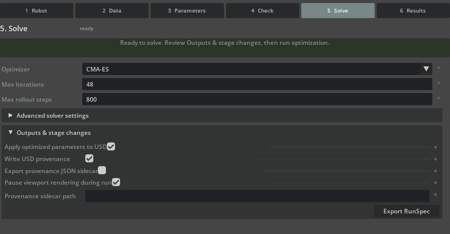
Review the writeback flags before exporting. Apply optimized parameters to USD and Write USD provenance are selected by default.#
Review every input path, output path, bound, and writeback flag. Point input paths at your local copies of
franka_sysid_tutorial/assets/franka_poor_seed.usda, franka_sysid_tutorial/data/bag_0.mcap,
franka_sysid_tutorial/data/franka_sysid_topic_map.yaml, and
franka_sysid_tutorial/data/collection_manifest.json. Keep output paths local. Store the exported file
with its topic mapping, collection manifest, source revision, and input hashes.
Step 8: Establish the poor-seed baseline#
Run the analyzer before optimization. Every command from here on reads its inputs from the packaged
subdirectories of your working directory copy and writes everything new into runs, so no command
overwrites a Samples original. Run them from the root of your NVIDIA Isaac Sim source checkout.
./_build/linux-x86_64/release/python.sh \
    source/extensions/isaacsim.robot_setup.sysid/tools/headless_sysid_analyze.py \
    --run-spec ~/sysid_tutorial/runs/franka_friction_run_spec.json \
    --stage ~/sysid_tutorial/assets/franka_poor_seed.usda \
    --result-json ~/sysid_tutorial/runs/poor_seed_baseline.json \
    --mode baseline
.\_build\windows-x86_64\release\python.bat `
    source\extensions\isaacsim.robot_setup.sysid\tools\headless_sysid_analyze.py `
    --run-spec C:\sysid_tutorial\runs\franka_friction_run_spec.json `
    --stage C:\sysid_tutorial\assets\franka_poor_seed.usda `
    --result-json C:\sysid_tutorial\runs\poor_seed_baseline.json `
    --mode baseline
The aligned held-out baseline was:
Metric |
Value |
|---|---|
Normalized cost |
0.008066 |
Position RMSE |
0.004443 rad |
Velocity RMSE |
0.017925 rad/s |
Torque RMSE |
2.1922 N*m |
Keep this report unchanged. A post-solve value without the same-stage, same-RunSpec baseline cannot establish improvement.
Step 9: Solve, then apply to a new USD#
Run the exported specification:
./_build/linux-x86_64/release/python.sh \
    source/extensions/isaacsim.robot_setup.sysid/tools/headless_sysid_solve.py \
    --run-spec ~/sysid_tutorial/runs/franka_friction_run_spec.json \
    --result-json ~/sysid_tutorial/runs/franka_friction_result.json \
    --checkpoint-json ~/sysid_tutorial/runs/franka_friction_checkpoint.json
.\_build\windows-x86_64\release\python.bat `
    source\extensions\isaacsim.robot_setup.sysid\tools\headless_sysid_solve.py `
    --run-spec C:\sysid_tutorial\runs\franka_friction_run_spec.json `
    --result-json C:\sysid_tutorial\runs\franka_friction_result.json `
    --checkpoint-json C:\sysid_tutorial\runs\franka_friction_checkpoint.json
Note
The exported RunSpec leaves Apply optimized parameters to USD and Write USD provenance
enabled, so this solve does author the selected values onto the stage it opens. Nothing reaches disk,
because writing the stage is gated separately by --save-stage, which the command above omits. That
is why the asset mutation in the next command is still an independent, reviewable step. The packaged
config/franka_friction_run_spec.json ships with both flags cleared; either setting reproduces the
result below, since the flags do not affect the optimization itself.
The selected candidate was the last accepted candidate at iteration 47. Review selected_status rather
than assuming the final attempted generation is accepted. The selected scales were:
Joint |
Initial scale |
Recovered scale |
Bound status |
|---|---|---|---|
Joint 1 |
1.000 |
0.214 |
Interior |
Joint 2 |
1.000 |
0.105 |
Interior |
Joint 3 |
1.000 |
0.848 |
Interior |
Joint 4 |
1.000 |
0.184 |
Interior |
Joint 5 |
1.000 |
0.172 |
Interior |
Joint 6 |
1.000 |
0.147 |
Interior |
Joint 7 |
1.000 |
0.156 |
Interior |
No selected value is classified as a bound hit. Joint 2 is close to the lower bound, so extending the search range would be a useful sensitivity study before interpreting its value physically.
Author the selected vector onto a new stage:
./_build/linux-x86_64/release/python.sh \
    source/extensions/isaacsim.robot_setup.sysid/tools/headless_sysid_apply_theta_to_stage.py \
    --run-spec ~/sysid_tutorial/runs/franka_friction_run_spec.json \
    --result-json ~/sysid_tutorial/runs/franka_friction_result.json \
    --stage ~/sysid_tutorial/assets/franka_poor_seed.usda \
    --output-stage ~/sysid_tutorial/runs/franka_friction_candidate.usda \
    --summary-json ~/sysid_tutorial/runs/franka_friction_apply_summary.json
.\_build\windows-x86_64\release\python.bat `
    source\extensions\isaacsim.robot_setup.sysid\tools\headless_sysid_apply_theta_to_stage.py `
    --run-spec C:\sysid_tutorial\runs\franka_friction_run_spec.json `
    --result-json C:\sysid_tutorial\runs\franka_friction_result.json `
    --stage C:\sysid_tutorial\assets\franka_poor_seed.usda `
    --output-stage C:\sysid_tutorial\runs\franka_friction_candidate.usda `
    --summary-json C:\sysid_tutorial\runs\franka_friction_apply_summary.json
This keeps optimization, asset mutation, and acceptance separately reviewable.
Step 10: Reload and compare held-out metrics#
Reload the persisted candidate in a fresh process and run a no-op baseline analysis:
./_build/linux-x86_64/release/python.sh \
    source/extensions/isaacsim.robot_setup.sysid/tools/headless_sysid_analyze.py \
    --run-spec ~/sysid_tutorial/runs/franka_friction_run_spec.json \
    --stage ~/sysid_tutorial/runs/franka_friction_candidate.usda \
    --result-json ~/sysid_tutorial/runs/franka_candidate_replay.json \
    --mode baseline
.\_build\windows-x86_64\release\python.bat `
    source\extensions\isaacsim.robot_setup.sysid\tools\headless_sysid_analyze.py `
    --run-spec C:\sysid_tutorial\runs\franka_friction_run_spec.json `
    --stage C:\sysid_tutorial\runs\franka_friction_candidate.usda `
    --result-json C:\sysid_tutorial\runs\franka_candidate_replay.json `
    --mode baseline
The independently reloaded candidate produced:
Held-out metric |
Poor seed |
Persisted candidate |
Change |
|---|---|---|---|
Normalized cost |
0.008066 |
0.004620 |
42.7% lower |
Position RMSE |
0.004443 rad |
0.004073 rad |
8.3% lower |
Velocity RMSE |
0.017925 rad/s |
0.015476 rad/s |
13.7% lower |
Torque RMSE |
2.1922 N*m |
1.6573 N*m |
24.4% lower |

The left panel normalizes each error channel by its own poor-seed value. The right panel shows the large scale correction produced by the deliberately over-frictional initialization.#
Inspect time-series agreement as well as aggregate values:

The persisted candidate follows the held-out position motion across all seven joints. Look for phase error, bias, and localized divergence that an aggregate RMSE can hide.#

Torque RMSE improves substantially but remains higher in absolute units than the state-channel RMSE. Residual effort error can include model-form, controller, effort-calibration, unmodeled friction, and timing mismatch; friction-only fitting is not expected to remove all of it.#
Step 11: Diagnose the residual and declare the next gate#
The friction candidate passes the first-phase fit gate because normalized cost and all three aggregate held-out channels improve after the result is persisted and reloaded. The effort overlay still contains structured amplitude and bias error, however. A tuning cycle should use that residual to form a new, testable phase rather than adding every available parameter at once.
For this tutorial, define an illustrative torque-refinement gate before running the second solve:
Requirement |
Gate |
|---|---|
Persisted-stage normalized cost |
Lower than the friction candidate |
Persisted-stage torque RMSE |
At least 10% lower than the friction candidate |
Position and velocity RMSE |
No more than 2.5% higher than the friction candidate |
Parameter bounds |
No selected bound hits |
Evidence source |
Fresh-process replay of the written USD |
These thresholds demonstrate the mechanism; define application-specific tolerances before fitting your own robot. A strict Pareto policy would instead reject any candidate that worsens any channel.
Duplicate the friction RunSpec and change its source stage to runs/franka_friction_candidate.usda. To
build the second contract in the panel, open runs/franka_friction_candidate.usda and repeat Steps 2
through 7 with two changes.
On 3 Parameters, click Clear all, then click Damping in the Families row and apply these bounds in Family bounds. Damping is a Solver calibration row in each joint group, not a Physical (SysID) row:
Family |
Count |
Initial |
Minimum |
Maximum |
|---|---|---|---|---|
Joint damping |
7 |
1.0 |
0.5 |
1.5 |
On 5 Solve, change CMA-ES sigma to 0.15 and CMA-ES seed to 20260731 under Advanced solver
settings. Keep the telemetry, chunks, command alignment, backend, controller, channel weights,
Max iterations of 48, and CMA-ES batch size of 16 unchanged. Export the new contract to
runs/franka_damping_run_spec.json, and add "cma_population_size": 16 to its solver section as
in Step 7.
Important
4 Check does not reach an ok verdict for a damping-only phase, and it is not supposed to. With
the seven damping scales selected, the presolve collapses to rank 0/0, condition inf (target:
unavailable), every verdict returns unknown, the report is not ok, and the Run button
stays disabled with Check reported blocking issues - resolve them and re-run Check before solving.
The reason is physical rather than a configuration error: drive damping does not appear in the
link-side torque equation at the true trajectory, so the analytical presolve has no column to rank it
with, and a family it cannot score keeps the unknown verdict that in turn withholds ok. The
optimizer identifies damping through simulated position response instead, which the presolve cannot
see.
Export RunSpec is unaffected, so export the contract from this closed-gate state and run the phase
headlessly in Step 12. Do not expect the ok badge from Step 6 or the ready badge from Step 7
here; both describe the friction phase only.
Run a local sensitivity analysis before optimizing:
./_build/linux-x86_64/release/python.sh \
    source/extensions/isaacsim.robot_setup.sysid/tools/headless_sysid_analyze.py \
    --run-spec ~/sysid_tutorial/runs/franka_damping_run_spec.json \
    --stage ~/sysid_tutorial/runs/franka_friction_candidate.usda \
    --result-json ~/sysid_tutorial/runs/damping_baseline_sensitivity.json \
    --mode sensitivity
.\_build\windows-x86_64\release\python.bat `
    source\extensions\isaacsim.robot_setup.sysid\tools\headless_sysid_analyze.py `
    --run-spec C:\sysid_tutorial\runs\franka_damping_run_spec.json `
    --stage C:\sysid_tutorial\runs\franka_friction_candidate.usda `
    --result-json C:\sysid_tutorial\runs\damping_baseline_sensitivity.json `
    --mode sensitivity
All seven reference perturbations produced non-low sensitivity and matching train/validation gradient signs. This is the evidence that justifies the trial despite the closed check gate: the analytical presolve cannot score damping, but a numerical perturbation still moves the simulated response measurably. Sensitivity supports a conservative trial, but it is not proof of unique physical identification.
Step 12: Solve, persist, and replay the damping phase#
Run the second RunSpec, again without --save-stage:
./_build/linux-x86_64/release/python.sh \
    source/extensions/isaacsim.robot_setup.sysid/tools/headless_sysid_solve.py \
    --run-spec ~/sysid_tutorial/runs/franka_damping_run_spec.json \
    --result-json ~/sysid_tutorial/runs/franka_damping_result.json \
    --checkpoint-json ~/sysid_tutorial/runs/franka_damping_checkpoint.json
.\_build\windows-x86_64\release\python.bat `
    source\extensions\isaacsim.robot_setup.sysid\tools\headless_sysid_solve.py `
    --run-spec C:\sysid_tutorial\runs\franka_damping_run_spec.json `
    --result-json C:\sysid_tutorial\runs\franka_damping_result.json `
    --checkpoint-json C:\sysid_tutorial\runs\franka_damping_checkpoint.json
The reference solve selected the last accepted candidate at iteration 33:
Joint |
Initial scale |
Selected scale |
Bound status |
|---|---|---|---|
Joint 1 |
1.000 |
1.290 |
Interior |
Joint 2 |
1.000 |
0.670 |
Interior |
Joint 3 |
1.000 |
0.923 |
Interior |
Joint 4 |
1.000 |
0.871 |
Interior |
Joint 5 |
1.000 |
0.567 |
Interior |
Joint 6 |
1.000 |
0.836 |
Interior |
Joint 7 |
1.000 |
0.579 |
Interior |
Write the selected vector to another new stage:
./_build/linux-x86_64/release/python.sh \
    source/extensions/isaacsim.robot_setup.sysid/tools/headless_sysid_apply_theta_to_stage.py \
    --run-spec ~/sysid_tutorial/runs/franka_damping_run_spec.json \
    --result-json ~/sysid_tutorial/runs/franka_damping_result.json \
    --stage ~/sysid_tutorial/runs/franka_friction_candidate.usda \
    --output-stage ~/sysid_tutorial/runs/franka_friction_damping_candidate.usda \
    --summary-json ~/sysid_tutorial/runs/franka_damping_apply_summary.json
.\_build\windows-x86_64\release\python.bat `
    source\extensions\isaacsim.robot_setup.sysid\tools\headless_sysid_apply_theta_to_stage.py `
    --run-spec C:\sysid_tutorial\runs\franka_damping_run_spec.json `
    --result-json C:\sysid_tutorial\runs\franka_damping_result.json `
    --stage C:\sysid_tutorial\runs\franka_friction_candidate.usda `
    --output-stage C:\sysid_tutorial\runs\franka_friction_damping_candidate.usda `
    --summary-json C:\sysid_tutorial\runs\franka_damping_apply_summary.json
Then reload the written stage in a new process:
./_build/linux-x86_64/release/python.sh \
    source/extensions/isaacsim.robot_setup.sysid/tools/headless_sysid_analyze.py \
    --run-spec ~/sysid_tutorial/runs/franka_damping_run_spec.json \
    --stage ~/sysid_tutorial/runs/franka_friction_damping_candidate.usda \
    --result-json ~/sysid_tutorial/runs/franka_damping_candidate_replay.json \
    --mode baseline
.\_build\windows-x86_64\release\python.bat `
    source\extensions\isaacsim.robot_setup.sysid\tools\headless_sysid_analyze.py `
    --run-spec C:\sysid_tutorial\runs\franka_damping_run_spec.json `
    --stage C:\sysid_tutorial\runs\franka_friction_damping_candidate.usda `
    --result-json C:\sysid_tutorial\runs\franka_damping_candidate_replay.json `
    --mode baseline
The optimizer’s paired in-process validation is valid candidate-selection evidence because it compares the authored and accepted values on identical chunks. It is not persistence evidence. Use the fresh-process replay report to prove that the saved layers compose the selected values and reproduce the expected motion.
Step 13: Compare the stages and choose the candidate#
The independently replayed stages produced:
Held-out metric |
Poor seed |
Friction candidate |
Friction+damping candidate |
|---|---|---|---|
Normalized cost |
0.008066 |
0.004620 |
0.003285 |
Position RMSE |
0.004443 rad |
0.004073 rad |
0.004153 rad |
Velocity RMSE |
0.017925 rad/s |
0.015476 rad/s |
0.015644 rad/s |
Torque RMSE |
2.1922 N*m |
1.6573 N*m |
1.3946 N*m |

The damping phase lowers aggregate cost and torque error, while position and velocity regress slightly relative to the friction-only candidate. All values come from independent persisted-stage replays.#
Relative to the friction candidate, the second phase lowers normalized cost by 28.9% and torque RMSE by 15.9%. Position and velocity RMSE increase by 2.0% and 1.1%. It passes the illustrative torque-refinement gate, but it does not strictly dominate the friction candidate.
Choose according to the policy declared in Step 11:
For torque-sensitive validation with the stated state-error tolerances, advance the friction+damping candidate to task-level testing.
For a strict no-regression policy or position-priority task, retain the friction-only candidate.
Preserve both stages. Promotion never requires overwriting the earlier accepted result.
Step 14: Decide whether another parameter phase is justified#
The second-stage report contains useful stopping evidence:
No damping scale hit a bound.
Parameter-confidence curvature was inconclusive for all seven damping scales.
Validation cost remained approximately 8.15 times the estimated noise floor.
Joint 2 retained the largest torque-residual power in the report.
Training and validation are still two segments of one multisine recording.
Do not respond by opening armature, link mass, center of mass, and inertia together on the same data. These families can explain overlapping acceleration-dependent residuals. Instead, collect independently designed motions: slow or static configurations for gravity terms, acceleration-rich segments for inertial terms, and a separate set of held-out frequencies. Then repeat the same cycle for one supported family at a time:
Establish the persisted-stage baseline.
Run the check and local sensitivity analysis.
Solve without
--save-stage.Apply the reviewed selected status to a new USD.
Replay the new stage in a fresh process.
Compare against the predeclared gate and retain or reject the stage.
For a separate known-truth algorithm and backend check, run Tutorial 15: Validate System Identification with Sim-to-Sim Recovery. That tutorial uses a simple double pendulum and transfers a Newton-recovered model into an NVIDIA Isaac Sim PhysX stage. It complements this recorded-data walkthrough; it does not turn the Franka fit into a known-truth result.
Step 15: Preserve evidence and decide#
Keep:
Source, poor-seed, and every candidate USD.
Recording, topic mapping, collection manifest, and declared train/validation split.
One exported RunSpec per parameter phase.
Baseline, sensitivity, result, checkpoint, apply summary, and independent replay reports.
Validation figures, acceptance policy, and any failed diagnostic reports.
Source revision, extension version, input hashes, GPU, driver, and optimizer seed.
The selected candidate is suitable for additional task validation only under the policy you declared before its solve. Keep the source USD untouched, and do not treat either tutorial outcome as a hardware-safety or physical-parameter certification.
Troubleshooting#
- Gravity feedforward does not support joint type …
The message names the Newton joint type and its model joint index, counted from
0at the root joint in articulation order. Feedforward supports revolute, prismatic, and fixed joints on a fixed base. Newton imports a fully locked generic USD joint as aD6joint with no free coordinates, which is treated as fixed. AFREEroot means the robot is floating-base, andBALLor partly lockedD6joints are not supported. Fix the named joint on the stage, or set Controller feedforward (simulation.newton.feedforward) tononefor that articulation.- Newton MuJoCo rollout diverged or
cudaErrorIllegalAddress(CUDA error 700) MuJoCo integrates drive stiffness explicitly. When a drive is too stiff for the inertia it moves, the rollout runs away within a few samples. Each candidate world is checked after every physics step; a diverged world is reset to its initial state and scored as an invalid candidate. If every world in a batch diverges, the rollout fails, and the message reports the stiffest drive, its joint path, and a minimum
simulation.newton.mujoco_substeps(MuJoCo substeps in the panel). Before raising the substep count, check the asset itself. USD angular drive stiffness is per degree, so a gain meant per radian is about 57 times too stiff. Implausibly small link inertias and missing joint armature lower the stable step as well. A CUDA error 700 with an older build has the same cause.- A headless tool printed an error but the shell reported success
Older builds discarded the tool’s exit status when shutting down NVIDIA Isaac Sim. The headless SysID tools now return a nonzero status when the run fails, so scripts can rely on the exit code.
Summary#
This tutorial covered:
Creating a controlled over-frictional working asset without modifying the source.
Declaring link-side torque semantics and correcting a measured 0.5361 s recording offset.
Separating coupled-multisine training and held-out frequency content.
Solving and independently replaying a bounded seven-friction phase.
Diagnosing the persisted residual before opening a second parameter family.
Solving and independently replaying a bounded seven-damping phase.
Comparing both candidates with an explicit application tradeoff.
Stopping when the existing excitation no longer supports a defensible broader solve.
Separating predictive fit quality from physical identifiability and known-truth validation.