


Holonomic Tutorial#
This tutorial demonstrates how to use HolonomicController to drive a
Kaya robot with full lateral mobility, using interactive sliders.
By the end of this tutorial, you’ll understand:
How
HolonomicControllercomputes per-wheel velocities from a body twistHow to place the control site with a pose, independently of the wheel geometry
How to use
HolonomicRobotUsdSetupto read wheel geometry directly from USDHow to provide a body-twist setpoint as a site
RobotState
Prerequisites
Review the Controllers and the RobotState tutorial to understand
the BaseController interface and RobotState.
To follow along, run:
./python.sh standalone_examples/api/isaacsim.robot_motion.controllers/holonomic.py

# ... or with the command site moved to the front of the wheel base
./python.sh standalone_examples/api/isaacsim.robot_motion.controllers/holonomic.py --front-control-point
Every code snippet below is taken from that script.
The script opens Isaac Sim with a Kaya on a flat stage and three slider windows, one per component of the body twist:
Slider |
Motion |
|---|---|
Forward speed (+x) |
Drive forward or backward |
Strafe speed (+y) |
Slide left or right without turning |
Yaw rate (+z) |
Rotate counter-clockwise or clockwise |
Unlike a differential drive base, all three are independent — set a forward speed and a strafe speed and a yaw rate at once and the robot does all three simultaneously.
How It Works#
You give the controller a body twist — a linear velocity \(v_c\) for the control site and a yaw rate \(\omega\) — and it works out how fast each wheel must spin. That happens in two steps.
First, how fast does each wheel need to move? The robot is rigid, so if the control site moves at \(v_c\) while the body turns at \(\omega\), the centre of wheel \(i\) travels at \(v_c + \omega \times r_i\), where \(r_i\) is that wheel’s position relative to the site. A wheel cannot move in every direction, though: spinning it drives the wheel centre along one axis, \(a_i\), while the rollers let it slide freely across that axis (both dependent on the mecanum angles). So only the component along \(a_i\) has to come from spinning the wheel:
Second, how fast must the joint turn to produce that? A wheel rolling without slipping moves its centre at radius × spin rate, so divide \(u_i\) by the wheel radius \(\rho_i\) — with one correction: on a mecanum wheel the rollers sit at an angle \(\gamma_i\), so only part of the wheel’s rotation drives along \(a_i\).
Wheel geometry#
The equations above use the following wheel directions. For wheel \(i\), express them in the command-site frame:
\(R_i\) is the rotational part of the pose of wheel \(i\) relative to the command-site frame.
\(s_i = \operatorname{normalize}(R_i\,\mathtt{wheel\_axis})\) is the positive wheel spin axis. Positive wheel speed follows the right-hand rule about \(s_i\).
\(n = \operatorname{normalize}(\mathtt{rotation\_direction})\) is the positive up and yaw axis.
\(d_i = \operatorname{normalize}(s_i \times n)\) is the positive rolling direction of the wheel disc.
The public input mecanum_angles[i] is \(\beta_i\), in degrees.
\(\beta_i\) is the right-handed angle about \(n\) from \(-s_i\) to
the roller’s long axis \(a_i\). At the ground contact, \(a_i\) is also
the no-slip direction. Equivalently,
where \(\operatorname{Rot}(n, \gamma_i)\) is a right-handed rotation about \(n\). Thus, \(\gamma_i\) is a derived roller offset, not the public mecanum-angle input. A value of \(\beta_i=90^\circ\) gives \(a_i=d_i\); \(45^\circ\) and \(135^\circ\) describe the two mecanum handednesses.
A free-spinning roller axis has no distinguished end. Interpret \(\beta_i\) modulo \(180^\circ\) in the range \([0^\circ,180^\circ)\); for example, \(-135^\circ\) and \(45^\circ\) describe the same roller geometry.
Define these directions at the roller that is at the bottom of the wheel and touching the ground. The figure shows a ground-plane projection of that same bottom-contact roller, not a roller at the top of the wheel.
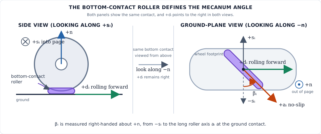
The mecanum angle is defined at the wheel’s bottom-contact roller.#
Both steps depend only on fixed geometry, so the controller works all of this out
once at construction and each forward() call is a small matrix multiply.
The Control Site#
Your setpoint is interpreted at the control site: \(v_c\) is the velocity of that point, and \(\omega\) turns the robot about it. When the controller is computing, every \(r_i\) above is measured from it too, so moving the site changes what the same command means.
As with the other controllers, the command is read from a named site in
setpoint_state.sites (control_point_name, default "control_point"),
and it is not the robot’s prim root — that sits wherever the USD author put it,
and the controller never looks at it.
What differs here is that you can choose where the site goes. A differential drive robot has a natural control point: the midpoint of its two wheels, the one point the kinematics actually solve for. An Ackermann vehicle has one too, fixed by which axle steers. A holonomic base has none — it translates and rotates freely, so no location is privileged by its geometry. The control site can be placed at any location whose velocity you want to command: the centre of the base body, a payload centre, or a camera mount.

The commanded twist applies here: \(v_c\) is this point’s velocity, and \(\omega\) turns the robot about it.#
Moving the Site#
Place it with command_site_position and command_site_quaternion,
expressed in the same frame you gave the wheel poses in. That is the only
rule. The site pose defaults to identity, which leaves the site at that frame’s origin —
for the Kaya, the centre of the wheel base. rotation_direction is read in
the site frame too, so its default [0, 0, 1] means the site’s own +Z.

Offsetting the site forward puts the commanded point out in front of the robot, so a yaw command swings the whole body around it instead of spinning in place.#
The example moves the site forward when using --front-control-point, marking the site
with a small red sphere. Run the example with and without the argument: with the
default site the robot spins on the spot; with the site moved forward the same
command sends it arcing around the marker.
Reading Wheel Geometry from USD#
Rather than measuring the wheels by hand, use HolonomicRobotUsdSetup
to read them from the authored USD prim attributes:
# Read the authored wheel geometry from the asset.
kaya_setup = HolonomicRobotUsdSetup(
    robot_prim_path="/World/Kaya",
    com_prim_path="/World/Kaya/base_link/control_offset",
)
wheel_radius, wheel_positions, wheel_orientations, mecanum_angles, wheel_axis, up_axis = (
    kaya_setup.get_holonomic_controller_params()
)
The helper measures everything relative to com_prim_path, so that prim’s
frame is the one your site pose is expressed in.
Note
This only works on an asset whose wheel geometry is authored in USD.
HolonomicRobotUsdSetup searches the robot prim’s subtree for joints
carrying an isaacmecanumwheel:angle attribute, then reads the roller angle
and the isaacmecanumwheel:radius from each one it finds. The Kaya ships
with both authored. On a robot that lacks them the helper finds no
wheels and raises, in which case measure the wheels yourself and pass
wheel_radius, wheel_positions, wheel_orientations, and
mecanum_angles to the controller directly.
Setting Up the Controller#
Pass the geometry returned by HolonomicRobotUsdSetup straight to the
controller constructor.
controller = ctrl.HolonomicController(
    robot_joint_space=list(my_kaya.dof_names),
    wheel_joint_names=WHEEL_JOINTS,
    wheel_radius=wheel_radius,
    wheel_positions=wheel_positions,
    wheel_orientations=wheel_orientations,
    mecanum_angles=mecanum_angles,  # authored per wheel; 90 on the Kaya, i.e. plain omni wheels
    wheel_axis=wheel_axis,
    rotation_direction=up_axis,
    command_site_position=command_site_position,
)
mecanum_angles comes from USD along with everything else — 90° per wheel on
the Kaya, and the X- or O-pattern angles on a true mecanum robot.
command_site_position above is what moves the site; the example computes it
from the wheel-base radius when you pass --front-control-point:
command_site_position = np.zeros(3)
if args.front_control_point:
    wheel_base_radius = float(np.max(np.linalg.norm(wheel_positions, axis=1)))
    command_site_position = np.array([FRONT_CONTROL_POINT_SCALE * wheel_base_radius, 0.0, 0.0])
Commanding a Velocity#
As with the other controllers, you state the motion you want the control site
to have and the wheels resolve the rest. Here that is a full planar twist —
[vx, vy, wz] — because a holonomic base can translate and rotate
independently:
site = "control_point"
setpoint = mg.RobotState(
    sites=mg.SpatialState.from_name(
        spatial_space=[site],
        linear_velocities=([site], wp.array([[command[0], command[1], 0.0]], dtype=wp.float32)),
        angular_velocities=([site], wp.array([[0.0, 0.0, command[2]]], dtype=wp.float32)),
    )
)
Running the Controller#
Call forward() every physics step and apply the resulting per-wheel
velocity targets:
desired = controller.forward(None, setpoint, 0.0)
if desired is not None and desired.joints is not None:
    my_kaya.set_dof_velocity_targets(
        desired.joints.velocities,
        dof_indices=my_kaya.get_dof_indices(desired.joints.velocity_names),
    )
get_dof_indices() maps joint names onto the articulation’s DOF ordering.
Derive the indices from desired.joints.velocity_names rather than from your
own WHEEL_JOINTS list: the values in desired.joints.velocities follow
the controller’s output ordering, and the two need not agree. The ordering is
fixed for the lifetime of the controller, so you can cache this lookup after
the first step instead of repeating it.

Kaya with the control site at the wheel-base centre (default).#

Kaya rotating around the translated control site (--front-control-point).#
Note
The Kaya model wheels cannot rotate at arbitrary speeds (it models a real robot). Therefore, if modifying the maximum linear and angular speeds in the python examples, keep in mind that the wheels may saturate.
Summary#
This tutorial demonstrated:
The control site: Placing it with a pose given in the wheel measurement frame
Wheel geometry from USD: Using
HolonomicRobotUsdSetupto avoid measuring by handMecanum angles: Setting 90° for omni wheels or per-wheel angles for mecanum layouts
Twist commands: Stating
[vx, vy, wz]for the site and letting the wheels resolve itOutput application: Mapping named velocity outputs back to joint indices
Next Steps#
Differential drive tutorial — simpler two-wheel controller
Ackermann tutorial — four-wheeled steering for car-like vehicles and forklifts